Introducing: CommodGrunt-Bench

My husband is really into benching, both the gym kind and the AI models kind. I got inspired and also wanted to see if it is possible to do this benchmarking thing for AI’s performance in commodities workflows.

First thing to be absolutely clear on, is that while there is already a very clear and quantifiable "bench" for commodities firms being PnL, this is not what I want to run evals on. Frankly because I don't believe AI can independently make PnL in the real world yet, and my exploration here is not about trading strategy backtesting.

What I want to measure is the performance of different agents on specific and clearly defined tasks which could contribute to PnL.

It was challenging to design a set of tasks to evaluate models on, for grunt work that could be universal across the industry. The tasks every analyst do might be similar (e.g. build and maintain Supply and Demand balances - SnDs), but every company has their own systems, workflows, and data pipelines etc. For a start, I decided to just go ahead and bench on a hypothetical SnD updating task where an analyst has to check a website for information.

An Essential but Tedious Task: Maintaining an SnD

Maintaining a SnD and keeping it updated is one of the daily tasks expected of a commodities analyst as a core tool for fundamental analysis, to quantify deficits and surpluses for commercial decisions. We look at Gas SnD as an example.

What a Gas SnD can look like:

Supply:
+ Pipelines
+ LNG Sendouts
+ Domestic Productions

Demand:
- Residential
- Power
- Industry
- Exports

Supply - Demand: Storage Injections/Withdrawal

There are many exciting factors which could move a Gas SnD:

• e.g. Outage at Freeport -> lower US LNG Exports -> lower Global LNG Supply -> lower expected LNG receipts at destination countries (depending on cargo allocation) -> thus feeding into model for a different storage path
• e.g. Increase in LNG Demand from China -> fewer flexible cargoes for Europe -> JKM may strengthen vs TTF -> Europe need higher TTF to attract cargoes -> Europe LNG receipts drop unless TTF price increases -> thus feeding into model for lower LNG supply into Europe

Outside of these event driven SnD movers, there are also the constant arrivals of LNG cargoes which needs to be updated in the LNG Sendouts section of gas balances, using LNG shipping data (AIS, port calls, nominations, regas terminal notices) on a daily basis. How each firm connects their balances to LNG shipping data is different, but hypothetically, this could be where daily grunt work lies.

Updating LNG Sendouts with LNG Shipping Data

The task of updating the LNG Sendout section of a gas balance using LNG shipping data could be broken down into 3 main steps:

1. Step 1: Checking the data source to identify the relevant vessels for our concerned regas terminals, respecting data cutoff standardisations.
2. Step 2: Comparing the portal records with the existing records in the excel SnD, and deciding whether each cargo should be added, updated, kept, excluded, or left unresolved.
3. Step 3: Updating the excel SnD correctly.

In summary, we are assessing whether AI can update the LNG supply part of a European gas SnD from the below data:

vessel / cargo observations
+ terminal operational data
+ nominations / sendout logic
+ prior Excel gas balance

Where most of the decision making sits in Step 2.

Walk through Step 2: from cargo records to LNG sendout

Step 2 is the decision-making part of the job. The analyst reads FlowScope and the prior cargo book, and decides what the schedule should contain

The physical LNG chain

LNG vessel → Terminal tanks → Regasification → Gas grid

A ship arriving does not immediately add gas supply to the European grid. The cargo first discharges into the terminal's LNG tanks. It only enters the gas balance when the terminal regasifies the LNG and sends the gas into the pipeline system.

Closing terminal inventory = opening inventory + LNG discharged − LNG sent into the grid − reloads − losses

This is why the model keeps a discharge date and a sendout-start date. They are normally the same gas day, but a terminal outage can separate them.

How sendout is calculated

Each included discharge leg gets the terminal's standard three-day sendout profile: 20% on Day 0, 50% on Day 1, and 30% on Day 2.

Leg energy = total cargo GWh × discharge fraction

A 600 GWh cargo starting sendout on 15 January therefore contributes 120 GWh on 15 January, 300 GWh on 16 January, and 180 GWh on 17 January. The three days add back to the full 600 GWh.

European gas days begin at 06:00 local terminal time. The analyst converts the UTC arrival into local time and assigns it to the gas day containing it. Unless a terminal notice says otherwise, sendout begins on that arrival gas day.

How the analyst works through the records

1. Freeze the information set. Use only records received by FlowScope at or before 12:00 UTC on 14 January. The received time matters, not when the underlying event happened.
2. Read the model scope. Dunkerque, Zeebrugge, South Hook, and Gate are included. Aliaga and Bilbao are outside the balance.
3. Read the prior cargo book. Match FlowScope records to existing cargoes using IMO and voyage ID.
4. Remove duplicates. Two feeds reporting the same vessel, voyage, event, time, and value are still one physical cargo.
5. Rank the evidence. A current terminal nomination outranks a confirmed port call, which outranks AIS destination text. AIS can support the vessel's laden state, but its destination may be stale.
6. Choose the disposition. Each material cargo becomes an add, update, confirm, exclude, or unresolved decision.
7. Set the legs and timing. Record the terminal, discharge date, sendout start, total cargo energy, discharge fraction, and whether it enters the balance.
8. Keep the audit trail. Cite the FlowScope record IDs and explain the decision in one or two sentences.

The nine cargo decisions

ALBA — add

ALBA is not in the prior book. Nomination obs-101 schedules 600 GWh at Dunkerque on 15 January, while AIS record obs-102 shows the same vessel and voyage laden and heading there. The standard sendout is 120, 300, and 180 GWh across 15–17 January.

CALYPSO — update

CALYPSO is already booked as cargo-201 for 15 January. Nomination obs-201 moves the 900 GWh Zeebrugge discharge to 17 January. The old profile must eventually be replaced by 180, 450, and 270 GWh across 17–19 January.

DELTA — exclude

DELTA was previously included at Dunkerque. Port-call record obs-301 confirms a diversion to Aliaga on 16 January. Aliaga is outside the model, so the analyst keeps the 750 GWh physical leg for audit purposes but sets include to No. It contributes no European LNG sendout.

BOREAL — confirm

An old AIS record says Southampton, but it is stale. Current nomination obs-402 confirms 600 GWh at Zeebrugge on 15 January. The nomination wins and the prior-book values stand. Its sendout remains 120, 300, and 180 GWh across 15–17 January.

EQUINOX — update into two legs

EQUINOX was previously one 1,000 GWh Dunkerque cargo. Records obs-501 and obs-502 show one voyage split across two terminals: 40% at Dunkerque on 15 January and 60% at South Hook on 17 January.

• The Dunkerque leg is 400 GWh and sends out 80, 200, and 120 GWh across 15–17 January.
• The South Hook leg is 600 GWh and sends out 120, 300, and 180 GWh across 17–19 January.

The JSON stores the 1,000 GWh cargo total on both legs and uses fractions of 0.4 and 0.6. It must not turn the legs into two separate cargoes.

FJORD — add, with delayed sendout

Nomination obs-601 schedules an 800 GWh discharge at Gate on 15 January. Notice cap-nl-20260115 reduces Gate's regasification capacity to zero for that gas day. The cargo still enters the terminal tanks on 15 January, but sendout starts on 16 January. The full profile shifts to 160, 400, and 240 GWh across 16–18 January.

MERIDIAN — add once

obs-701 and obs-702 are duplicate AIS reports from two feeds. Nomination obs-703 provides the controlling 500 GWh Dunkerque schedule. The analyst adds one cargo, producing 100, 250, and 150 GWh of sendout across 15–17 January.

GALLANT — update using the cutoff-correct record

obs-801, received at 10:01, moves the 700 GWh cargo to 16 January. A later correction, obs-802, says 15 January but was not received until 12:30. It falls outside the information cutoff and must be ignored, even though its event time is 11:55. The accepted profile is 140, 350, and 210 GWh across 16–18 January.

HELIOS — unresolved

obs-1001 nominates Dunkerque while obs-1002 nominates Zeebrugge. They are equal-priority records, and FlowScope provides no tie-break. The quantity is also given as 170,000 m³ of liquid LNG, while the model provides no conversion from liquid volume to GWh. The analyst leaves the cargo out of the numerical balance and explains both problems.

The workbook's 10.8 GWh per mcm assumption cannot solve the HELIOS case. It converts a standard volume of gaseous natural gas into energy; it is not a conversion for cubic metres of cryogenic liquid LNG.

What the decisions do to the balance

Terminal	Included tracked energy
Dunkerque	1,500 GWh
Zeebrugge	2,200 GWh
South Hook	600 GWh
Gate	800 GWh
Total	5,100 GWh

The prior book contains 3,950 GWh, so the decisions add a net 1,150 GWh to January. The workbook also carries 2,200 GWh/day of base LNG sendout. That gives 68,200 GWh of base sendout plus 5,100 GWh from the tracked cargoes, or 73,300 GWh for January.

January LNG supply = 73,300 GWh ÷ 31 days ÷ 10.8 GWh/mcm = 218.94 mcm/d

That sendout feeds total European gas supply. With demand at 635 mcm/d, the remaining gap is about 16.06 mcm/d of storage withdrawal. Task 02 does not calculate or write those spreadsheet outputs, but its cargo decisions determine them.

Setting up the Exam Paper

Models were evaluated running inside the same Pi agent.

They were provided two things:

1) a European gas balance Excel workbook

The workbook starts with the previous day’s LNG cargo schedule. The agent updates the editable cargo fields: terminal, discharge date, sendout start, cargo size, discharge fraction, inclusion status, and evidence IDs. Formulas then spread each included cargo across its three-day sendout profile, roll the LNG through terminal inventory, and convert total terminal sendout into the monthly European gas balance. The agent also completes the Update Log so every change can be traced back to FlowScope.

Download the starting Excel workbook to see the file supplied to the agent before it makes any updates.

2) a link to the FlowScope web page: A made-up LNG data portal containing pages for vessels, cargoes, terminals, notices, and methodology.

A made-up web page containing synthetic data with intentional ambiguities to trip up models. There are stale vessel positions, duplicate-looking records, split discharges, terminal constraints, and an unresolved cargo whose units cannot be safely converted with the information provided. The correct response is sometimes to update a number. At other times, it is to leave the workbook alone and record why.

Open FlowScope to browse the same vessel, cargo, terminal, notice, and methodology pages used in the eval.

The 3 main steps (Step 1-3) discussed above were organised into independent tasks so each could be evaluated in isolation (no cascading outputs), with a fourth task defined as being the actual full update task:

1. Task 01: vessel reconnaissance. Read FlowScope, identify the relevant inbound cargoes, respect the information cutoff, and return the supporting record IDs as structured JSON.
2. Task 02: cargo reconciliation. Compare the portal records with the prior cargo book and decide whether each cargo should be added, updated, kept, excluded, or left unresolved. This is also returned as structured JSON.
3. Task 03: Excel execution. Take a supplied, reviewed set of cargo decisions and apply it to the workbook without breaking its formulas. The decisions are deliberately provided so this task tests spreadsheet execution on its own. An agent can fail Task 02 and still pass Task 03.
4. Task 04: full update. Do the complete job: read the portal, make the reconciliation decisions, update the workbook, preserve the formulas, document the evidence, and save a working .xlsx file.

That split helps show where an agent fails. It may be good at reading the website but poor at reconciliation. It may reach the right commercial decision but damage the spreadsheet. Task 04 is therefore the headline end-to-end result; Tasks 01–03 explain why an agent succeeded or failed.

Judging Criteria

The grading is deterministic. There is no language model deciding whether the answer feels right.

For the first two tasks, the agent returns structured JSON. The grader checks it against frozen reference data, including the allowed records, timestamps, decisions, and evidence.

For the workbook tasks, the grader opens the submitted .xlsx file and checks the contents directly. The full task is scored across five areas:

• the operational schedule: 40 points;
• the numerical gas balance: 25 points;
• evidence and cutoff discipline: 20 points;
• workbook integrity: 10 points;
• handling uncertainty correctly: 5 points.

There are also penalties for serious failures, such as adding unsupported cargo legs or changing cells that should have remained formulas.

Results

From 11 to 14 August 2026, with the help of my husband, we ran evals across eight models and all four tasks using Pi as the agent. Harbor supplied the tasks, isolated candidate environments, and deterministic verifiers.

A red outline below means the task failed. That can happen even when the numerical score is above 70% because a critical error (e.g. an unsupported cargo or a damaged workbook formula) overrides the score.

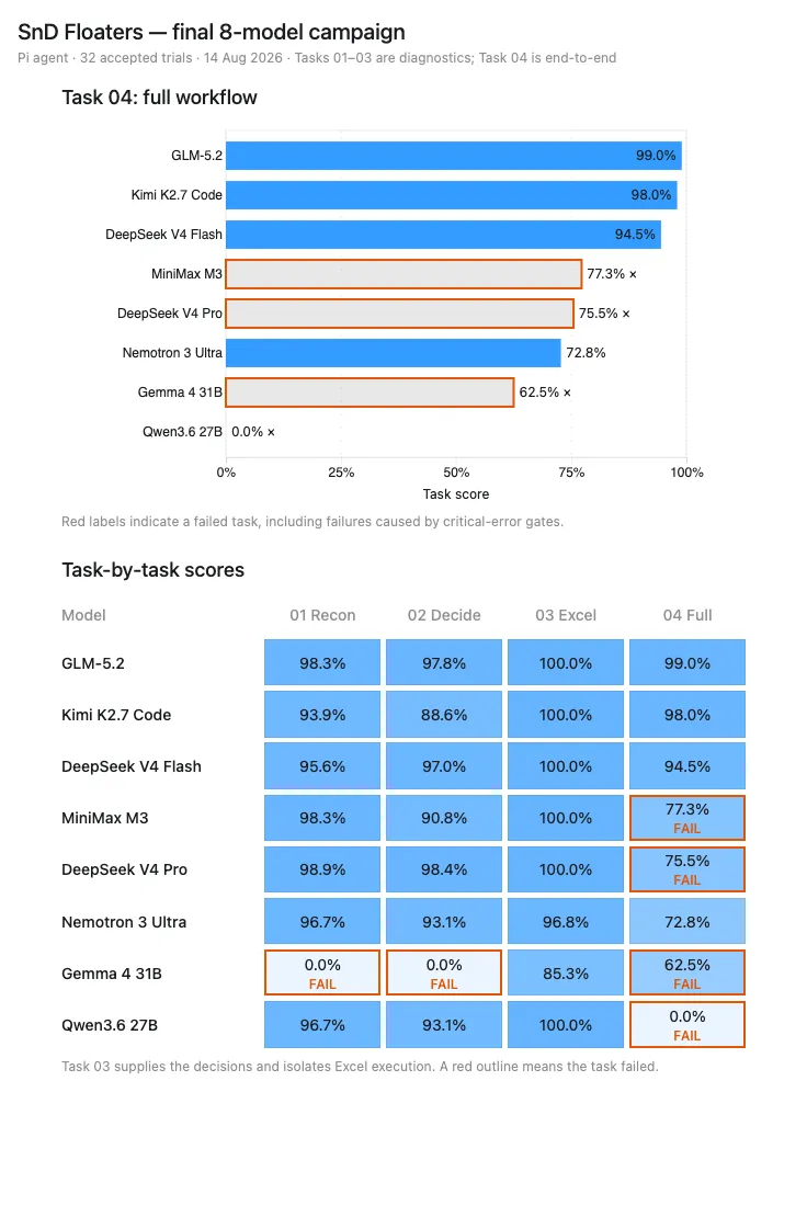The diagnostic split is visible in the results. Task 03 was consistently strong because the decisions were supplied and the agent only had to execute them in Excel. Task 04 separated the models much more clearly because it required the complete workflow. GLM-5.2, Kimi K2.7 Code, and DeepSeek V4 Flash were the strongest end-to-end performers in this campaign.

Though, in this campaign each task for each model was ran only once. E.g. in the “Task-by-task scores” table, DeepSeek V4 Pro’s 98.4% on Task 02 came from a single trial. A more reliable comparison would run every model on each task several times, then report the average score and pass rate but that would burn a lot of tokens.

It was also interesting to observe the run-to-run variation from this. DeepSeek V4 Pro was particularly interesting: it had performed well for Task 01-03, but fumbled on the run for Task 04 as it failed to apply the cutoff consistently. In critical commercial workflows, run-to-run variations like these are unacceptable, and if an Agent is actually used, it has to demonstrate much better consistency.

What Benchmarks for Commodities workflows should be about

The interesting question is not simply whether an agent can use a browser or edit Excel. It is whether it can combine several kinds of judgment in one controlled workflow:

• find the relevant information;
• respect a point-in-time cutoff;
• reconcile conflicting records;
• distinguish a safe update from an unresolved case;
• modify an existing model without damaging it;
• leave enough evidence for a human to audit the result.

The larger goal is to make evaluations look more like the work we actually care about. In commodity research, the value of an answer is not just that the final number is correct. It is that the path to the number is timely, traceable, and safe to use in the next decision.

Appendix: Bench Design Lessons

A lesson from building this eval is that a realistic task is not enough. The grader also needs to resist shortcuts.

For example, an answer should not receive full credit if it includes the required cargoes plus several invented ones. A workbook should not pass just because a few headline cells match the reference while its formulas or update log are missing. JSON timestamps need to be checked as real timestamps, not merely as strings that look roughly right.

I tightened those areas and added adversarial tests for malformed JSON, duplicate records, extra cargo legs, incomplete update logs, and overwritten formulas.

This is less glamorous than designing the task, but it may be the most important part. A benchmark measures whatever its grader rewards. If the grader leaves a loophole, the score can stop meaning what we think it means.